This project looked at tweets from "We Rate Dogs" over a period of 624 days from November 2015 until August 2017. These tweets are often accompanied by pictures as well as ratings. Not all pictures and posts concern dogs, but most do. Ratings are usually given as a score out of 10. The ratings, famously, are allowed to surpass 10, however. So, a rating of 12/10 is not uncommon. Sometimes, more than one dog is the subject of the tweet in which case the rating may be a score out of some multiple of 10 depending on the number of dogs involved. The ratings are not intended to be taken too seriously and are sometimes the subject of much joking in the replies to the tweets.
The names of the dogs are sometimes included in the text of the tweets. These names can be scraped from the text. For this period, the four most popular names appearing in the tweets were: 'Charlie', 'Oliver', 'Lucy', and 'Cooper'.
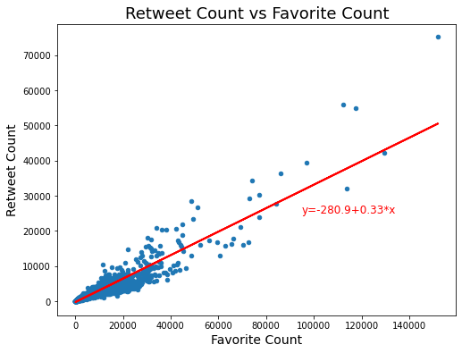
Tweets get both retweeted and favorited. One might expect the retweet_count to be strongly correlated with the favorite_count since both would seem to be measures of popularity. Indeed, this is the case with a correlation coefficient of 0.926 which corresponds to a R-squared value of 0.857. So, the two features favorite_count and retweet_count are strongly positively correlated, as one might expect.
The following is a plot of retweet_count versus favorite_count with the linear regression line added.
As noted already, "We Rate Dogs" provides ratings as a ratio with a non-negative numerator and a denominator that is often 10 or some multiple of 10 -- for example "13/10". When the denominator is some multiple of 10, it is almost always because more than one dog is involved in the picture(s). For what follows, we exclude cases with multiple dogs as best we can by only looking at ratings where the denominator is 10. (This technique is not a perfect filter for just posts about a single dog since sometimes a rating might be give as "12/10 for each one". But at least in that case the rating is clearly meant to apply to each individual rather than to the group in aggregate.) By selecting posts only where the denominator is 10, we can summarize the rating easily by simply looking at the rating numerator alone.
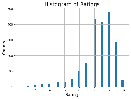
With a count of 2087 ratings, the mean rating was 10.6 and the median 11. The bulk of the ratings (in fact, the three upper quartiles) were greater than or equal to 10. This is evident in the histogram below which shows a left-skewed distribution.
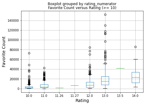
Is there any relationship between favorite_count and rating? Below, we see that higher favorite counts are associated with higher ratings.
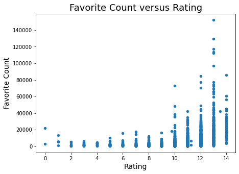
The distribution plotted above also shows that there is something of a "discontinuity" (loosely-speaking) at the 10 rating. The value of 10 bifurcates the ratings into two groups: < 10 and >= 10. We saw previously that the number of ratings increases substantially at 10. Plus, we see here that higher frequency counts only occur for ratings greater than or equal to 10. So, in examining favorite count versus rating further, the data was divided according to this natural bifurcation.
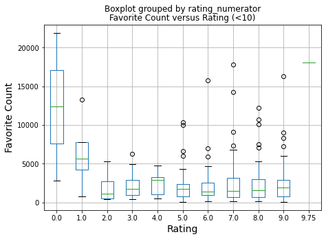
Here we see that for ratings < 10, most tweets are favorited less than 5000 times. Of course, there are also less tweets that receive these lower ratings. The distribution for our data is given below.
| Rating | Number of Tweets |
|---|---|
| 0.00 | 2 |
| 1.00 | 4 |
| 2.00 | 9 |
| 3.00 | 19 |
| 4.00 | 15 |
| 5.00 | 33 |
| 6.00 | 32 |
| 7.00 | 51 |
| 8.00 | 98 |
| 9.00 | 154 |
| 9.75 | 1 |
Looking at ratings >= 10, we see the box plots growing taller as the ratings increase. The highest range of the previous plot (20000) is only the first gradation of this one. Some tweets with these ratings achieve very hight favorite counts.
There are more tweets for these higher ratings. The distribution of tweets at the higher ratings is given here.
| Rating | Number of Tweets |
|---|---|
| 10.00 | 435 |
| 11.00 | 417 |
| 11.26 | 1 |
| 11.27 | 1 |
| 12.00 | 482 |
| 13.00 | 291 |
| 13.50 | 1 |
| 14.00 | 41 |
It was observed informally during data cleaning that low ratings sometimes indicate that a picture does not contain a dog but rather a different kind of animal (like a hedge hog, for example). This suggested that ratings could be used as an indicator for whether the post concerns a dog. Put as a question, "Does 'We Rate Dogs' use low ratings to indicate that the post is not about a dog?" Or more precisely, "How strong of an indicator is the rating for the presence of a dog in the post?" To answer this, we would need to know which posts concern a dog and which do not. Since that data was not readily available, we used the machine learning (ML) predictions data provided to us as a benchmark for whether a post concerns a dog. This is an imperfect benchmark, since the prediction data itself should be tested for reliability. So, the more accurate way of looking at this investigation is as a comparison of using the ratings as dog predictors with the machine learning prediction data provided. The ML prediction data provides three ranked predictions -- first, second, and third in confidence. We compared the ratings as dog predictors with (1) the top ranked predictions of the ML algorithm as well as with (2) the conjunction of the ranked predictions. The latter case is a conservative prediction and will only predict a dog when all three ranked predictions say there is a dog (i.e., the conjunction of the predictions); otherwise, the default is that there is not a dog.
Starting with 1973 posts with predictions, the ML algorithm's top ranked prediction yielded 1461 dogs and the conjunction of ranked predictions yielded 1189 dogs. We can see the distribution of those predictions -- "Dog" versus "No Dog" -- for each rating below as given by the top ranked (highest confidence) prediction for each tweet.
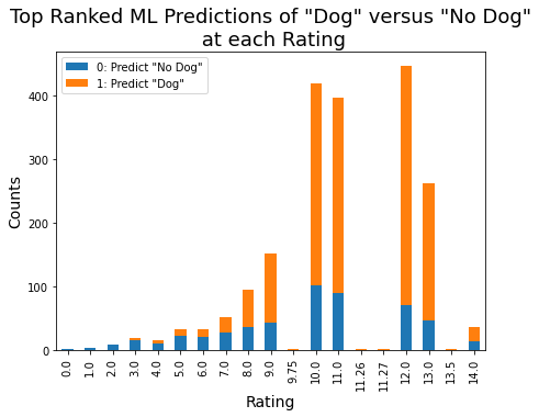
In the plot, the proportion of orange to blue per bar increases roughly as the ratings increase. This means that the proportion of ML predictions of "Dog" to "No Dog" increases roughly as the ratings increase. (Or, from the opposite perspective, lower ratings are stronger indicators of "No Dog".) This increase is particularly strong for ratings less than 10 and is less so (it appears to roughly flatten out) for ratings greater than or equal to 10.
This relationship suggests that the dog ratings themselves can be viewed somewhat as predictors of "Dog" versus "No Dog". This relationship was examined using logistic regression over a few cases:
1) Rating as a predictor of Top Ranked ML Dog Predictions
2) Rating as a predictor of the Conjunction of ML Dog Predictions
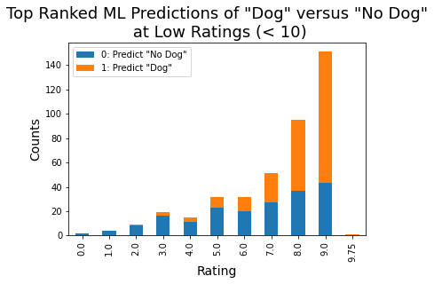
3) Rating as predictor of Top Ranked ML Dog Predictions for low ratings (< 10)
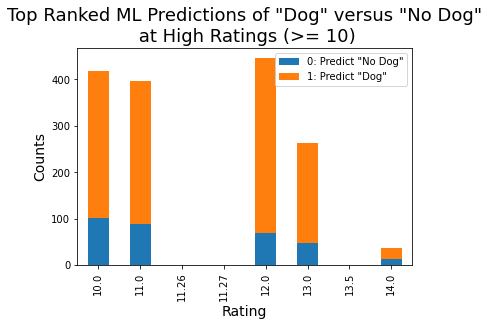
4) Rating as predictor of Top Ranked ML Dog Predictions for high ratings (>= 10)
The logistic models from the results of the logistic regressions are summarized in the following table. For full details (p-values, confidence intervals for the parameters, etc.) see the full analysis.
| Rating as a predictor of | Intercept | Rating Coefficient | Odds Ratio |
|---|---|---|---|
| Top Ranked ML Dog Predictions | −1.933 | 0.289 | 1.34 |
| Conjunction of ML Dog Predictions | −1.876 | 0.218 | 1.24 |
| Top Ranked ML Dog Predictions for low ratings (< 10) | −3.167 | 0.452 | 1.57 |
| Top Ranked ML Dog Predictions for high ratings (>= 10) | 0.239 | 0.0978 | 1.10 |
The logistic model in this situation with just a single independent variable is:
$log_e \Big( \frac{p_i}{1 - p_i} \Big) = \text{Intercept} + \text{Coefficient}\times \text{rating}$.
Where $ \frac{p_i}{1 - p_i} $ is the odds of the ML algorithm predicting a "Dog" given a particular $\text{rating}$, the odds ratio is
$\text{Odds Ratio} = \frac{\text{Odds given rating = x + 1}}{\text{Odds given rating = x}}$.
It can be shown that
$\text{Odds Ratio} = exp(\text{coeff. of rating})$.
So, in the first case, the model is
$log_e \Big( \frac{p_i}{1 - p_i} \Big) = −1.933 + 0.289\times \text{rating}$
so that in this first case the odds ratio is $exp(0.289) = 1.34$.
The odds ratio indicates that we expect a multiplicative change of 1.34 in the odds for an increase in rating by 1. In other words, the model predicts a 34% increase in the odds of the ML algorithm predicting a "Dog" for each increase in rating by 1.
Comparing the odds ratios allows us to interpret how well the ratings function as a predictor in the various cases. First, we see that the ratings track with the Top Ranked ML Dog Predictions (odds ratio = 1.34) a little better than with the Conjunction of the ML Dog Predictions (odds ratio = 1.24). Second, the change in ratings is more informative over the low ratings (odds ratio = 1.57) than over the high ratings (odds ratio = 1.10). Of course, we noticed this relationship visually from the previous stacked bar charts. The change in the proportion of "Dog" to "No Dog" predictions increased steadily over the lower ratings (< 10) as the ratings increased. However, it nearly flattened off for the higher ratings (>= 10).